RECENT POSTS
- Introducing modelx-cython: Boosting modelx with Cython Compilation
- A First Look at Python in Excel
- Enhanced Speed for Exported lifelib Models
- New Feature: Export Models as Self-contained Python Packages
- Why you should use modelx
- New MxDataView in spyder-modelx v0.13.0
- Building an object-oriented model with modelx
- Why dynamic ALM models are slow
- Running a heavy model while saving memory
- Running modelx in parallel using ipyparallel
- All posts ...
Introduction to fastlife and parallel modeling
Dec 12, 2020 • Fumito Hamamura
In one of my recent blog posts, I wrote about how I wanted to develop parallellife, a model that processes multiple model points in parallel. I finally got time to work on its prototype. The name parallellife is a bit too long, so I eventually named it fastlife. In this post, I discuss how different fastlife is from simplelife, how it performs, how I plan to improve its performance, and why the parallel modeling approach reduces modeling errors. Although it’s still premature, the fastlife prototype model can be downloaded from the link below so that you can play around with it and reproduce what’s written in this post.
The file can be read into an IPython session by lines like these:
>>> import modelx as mx

>>> fastlife = mx.read_model("fastlife-20201212.zip")
Model overview
The fastlife model outputs exactly what a simplelife model does, i.e. it calculates the present value of the net future cashflows of each model point. The difference is, while the simplelife model calculates the present value for one model point at a time, the fastlife model calculates the present values for all model points at once. Let me show you how this works in more details.
With a simplelife model, to get the present value of net cashflows for Policy 1, you can do:
>>> simplelife.Projection[1].PV_NetCashflow(0)
8954.018303162458
The Space Projection[1] is only for Policy 1, so to get the present values of net cashflows of all the 300 model points in a list, you can do:
>>> [simplelife.Projection[i].PV_NetCashflow(0) for i in range(1, 301)]
[8954.018303162458,
 7511.092085138853,
 9173.906589547994,
       ...
 2557190.764898183,
 2242406.3150801933,
 2510715.051976551]
On the other hand, the fastlife model returns the present values for all model points in a Series:
>>> fastlife.Projection.PV_NetCashflow(0)
1      8.954018e+03
2      7.511092e+03
3      9.173907e+03
4      7.638071e+03
5      9.418541e+03
          ...
296    2.599794e+06
297    2.298079e+06
298    2.557191e+06
299    2.242406e+06
300    2.510715e+06
Length: 300, dtype: float64
Note that the formulas of PV_NetCashflow in the two models are the exactly the same:
>>> simplelife.Projection[1].PV_NetCashflow.formula
def PV_NetCashflow(t):
    """Present value of net cashflow"""
    return (PV_PremIncome(t)
            + PV_ExpsTotal(t)
            + PV_BenefitTotal(t))

>>> fastlife.Projection.PV_NetCashflow.formula
def PV_NetCashflow(t):
    """Present value of net cashflow"""
    return (PV_PremIncome(t)
            + PV_ExpsTotal(t)
            + PV_BenefitTotal(t))
While the formula in the simplelife model operates on scalar values for a selected model point, the formula in the fastlife model operates on Series, which means
PV_PremIncome(t), PV_ExpsTotal(t), and PV_BenefitTotal(t) in the formula of PV_NetCashflow(t) in the fastlife model are all returning Series.
Performance
Now let’s see how fast a fastlife model is. The code below is for comparing execution time between the two models.
>>> import timeit

>>> timeit.timeit("[simplelife.Projection[i].PV_NetCashflow(0) for i in range(1, 301)]", number=1, globals=globals())
30.510370499999993

>>> timeit.timeit("fastlife.Projection.PV_NetCashflow(0)", number=1, globals=globals())
20.70127050000002
I had hoped that the fastlife model would gain extreme performance improvement as I wrote here, but the improvement is only about 30%. But, it’s too early to despair. It’s quite likely that the model’s performance improves drastically by making some changes for optimization. In the next section, I’m going to discuss how I inspected the fastlife model to identify performance bottlenecks.
Inspection and analysis
modelx has a stack trace feature, which enables you to see how much time each formula took during an execution. The code below keeps track of the execution information of formula calls while calculating the present values of the net cashflows.
>>> import modelx as mx

>>> mx.start_stacktrace(maxlen=None)
UserWarning: call stack trace activated
True

>>> fastlife.Projection.PV_NetCashflow(0)
Policy
1      8.954018e+03
2      7.511092e+03
3      9.173907e+03
4      7.638071e+03
5      9.418541e+03

296    2.599794e+06
297    2.298079e+06
298    2.557191e+06
299    2.242406e+06
300    2.510715e+06
Length: 300, dtype: float64

>>> import pandas as pd

>>> trace = mx.get_stacktrace(summarize=True)

>>> df = pd.DataFrame.from_dict(trace, orient="index")

>>> mx.stop_stacktrace()
True
df holds a DataFrame each record of which shows the name of a Cells (or a Space) object, how may times the formula of the object is executed, and how long the executions of the formula took in total.
The table below shows the top 5 Cells that took time the longest.
| calls | duration | |
|---|---|---|
fastlife.Projection.Assumptions.MortFactor(y) |
103 | 6.298937321 |
fastlife.Projection.Assumptions.SurrRate(y) |
103 | 6.012678623 |
fastlife.Projection.Policy.ReserveNLP_Rate(basis, t) |
104 | 5.720100403 |
fastlife.Projection.BaseMortRate(t) |
103 | 1.585314989 |
fastlife.Projection.BenefitTotal(t) |
103 | 0.213982344 |
You see that the fist 3 Cells took about 18 seconds in total. Since the entire execution duration, which is the sum of the 3rd column’s figures, is about 23 seconds, the 3 Cells account for more than 75% of the entire execution.
Let’s see the formula of fastlife.Projection.Assumptions.MortFactor, which is taking time the most.
>>> fastlife.Projection.Assumptions.MortFactor.formula
def MortFactor(y):
    """Mortality factor"""

    def get_factor(pol, y):

        key1, key2, key3 = pol['Product'], pol['PolicyType'], pol['Gen']
        table = AsmpLookup.match("MortFactor", key1, key2, key2).value

        if table is None:
            raise ValueError('MortFactor not found')

        result = AssumptionTables.get((table, y), None)

        if result is None:
            return MortFactor(y-1)[pol.name]
        else:
            return result


    return PolicyData.apply(lambda pol: get_factor(pol, y), axis=1)
fastlife.Projection.Assumptions.SurrRate, the second time-consuming formula looks similar to the above. These formulas apply functions that are defined in the formulas to PolicyData, a Pandas Series object. Within the functions applied to PolicyData,
the AsmpLookup.match method is called, which is algorithmically a pretty expensive operation. Getting rid of this method, and hopefully of the locally defined functions, get_factor all together should shorten the execution time by a lot if it’s all possible.
By inspecting time-consuming formulas like the above and finding ways to rewrite their code to optimize performance, I’m sure the performance of the fastlife model should improve significantly.
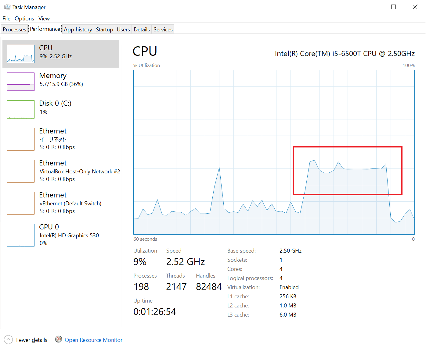
Analysis on parallelization
I also looked at how the fastlife model is utilizing CPU cores. As you can see in the following figure, it’s only utilizing about 30% or less, given 10% was used by other processes. This is because Pandas is not utilizing multi-threading, and it was not utilizing all the 4 cores on my PC.
Unfortunately, Python cannot benefit from multi-threading due to its mechanism called GIL. I looked around for a solution and found modin. In short, modin’s goal is to behave exactly like pandas but with multi-threading and/or multi-processing enabled. I quickly tested modin, but I couldn’t get it work with modelx. I believe I can make modelx work with modin, but need further study.
Other findings
Until I started working on the prototype, I had thought that writing formulas for all model points at a time (let’s name it parallel modeling ) would be much more difficult than writing it for just one model point, because you have to simultaneously think about all possible logic that any one of all the model points can take. As I proceeded with modeling the prototype by making changes to a simplelife model, I started feel like parallel modeling was not so hard. In fact, I felt like this way of modeling might be less error-prone than modeling for one model point at a time. Let me further explain why I think this is less error-prone. When you write a formula for one model point, you focus only on the logic of the formula that the chosen model point should take. Then you move on to another formula, and writes the formula for the same model point ignoring logic that other model points could take, then you repeat this routine for other formulas till you finish writing all the formulas relevant for the model point. You would then start modeling for other model points. Many of the formulas would be valid for many of the other model points without any changes, but some of the formulas need changes to incorporate logic that some of the model points can take. The logic can be for such model points that have different states at different times than the original model point. It also can be for such model points that have different policy features and options. Based on your knowledge on the products you’re modeling, you find formulas to make residual changes on. This sporadic manual process is error-prone. You’ll never be entirely sure when you finished covering all the formulas for all the model points. In contrast, parallel modeling forces you to consider all model points in scope when writing one formula. The formula operates on all the model points, so you can’t carry out the calculation only for a single model point or a subset of all the model points (Although technically you can by limiting model points in scope). This gives you great confidence when you finish writing the last relevant formula. When it’s done, it’s done for all the model points.
Conclusion
The fastlife prototype model is yet only 30% faster than simplelife. However, code optimization should improve its performance drastically. Further more, By integrating modelx with modin, fastlife should be able to utilize CPU cores in parallel, resulting in further performance improvement. The parallel modeling approach is expected to reduce modeling errors.