RECENT POSTS
- Introducing modelx-cython: Boosting modelx with Cython Compilation
- A First Look at Python in Excel
- Enhanced Speed for Exported lifelib Models
- New Feature: Export Models as Self-contained Python Packages
- Why you should use modelx
- New MxDataView in spyder-modelx v0.13.0
- Building an object-oriented model with modelx
- Why dynamic ALM models are slow
- Running a heavy model while saving memory
- Running modelx in parallel using ipyparallel
- All posts ...
Running a heavy model while saving memory
Mar 26, 2022
In a couple of earlier posts, modelx performance has been discussed. While modelx runs heavy actuarial models pretty fast, one issue with modelx was its massive memory consumption.
To address the issue, a new feature has been in development and it is soon to be added in a future release of modelx. This post discusses how the feature works and shows the result of its initial performance test.
The interface design of the feature has not finalized yet, and will be updated by its official introduction.
Update on 16 April 2022: modelx v0.19.0 introduced this feature. This post is updated to reflect the actual method names, generate_actions and execute_actions.
The issue with memory consumption
Let’s take lifelib’s CashValue_ME model for example.
Running the model with 100K model points consumes
up to 33 GB of additional memory (In the figure below, 9.5GB is consumed for other use).

This wouldn’t be a problem for a compute engine in a cloud environment, which has up to a few terabytes of memory, but common desktop PCs come with much less.
The reason why the run uses so much memory is that to calculate the target result you want in the end, modelx keeps all the intermediate results that are calculated indirectly by the formulas recursively referenced from the target formula.
The memory saving mechanism
The new feature carries out calculation in multiple steps. In each step, a specified number (1000 by default) of nodes are calculated. A node is a pair of a formula and its arguments. Nodes are topologically sorted so that the ones calculated in an earlier step don’t depend on those calculated in the later steps. The memory saving mechanism works by pasting the values of the nodes calculated in the earlier steps that are referenced by the ones calculated in later steps, and clearing the values of other nodes that are not referenced anymore.
To understand the mechanism better, let’s take this simple model for example.
import mx

@mx.defcells
def Cells1():
    return 1

@mx.defcells
def Cells2(x):
    if x > 0:
        return Cells2(x-1)
    else:
        return Cells1()

@mx.defcells
def Cells3(x):
    return Cells1() + Cells2(x)
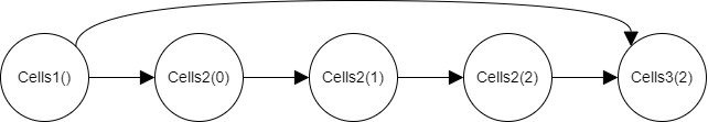
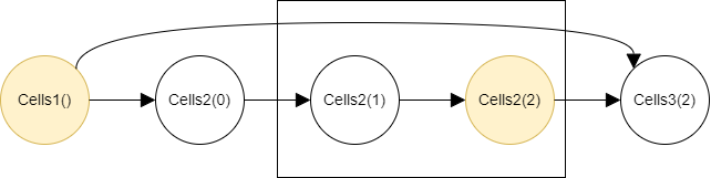
Let’s say your target node is Cells3(2).
Cells3(2) directly depends on Cells1() and Cells2(2),
and the whole dependency graph of the calculated nodes looks like below.
The nodes in the diagram below are in a topological sort order.
So any node in the diagram does not depend on those placed
on the right side to the node.
Let’s assume 2 nodes are calculated in each step.
Then in the first step, Cells1() and Cells2(0) are calculated.
The calculated nodes are highlighted in blue:
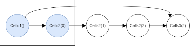
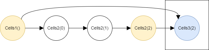
Then the both two nodes are value-pasted, as highlighted in yellow, because both have edges going out of the first step rectangle. Having such edges indicates that the two nodes are referenced in later steps, so the values of them need to be preserved now.
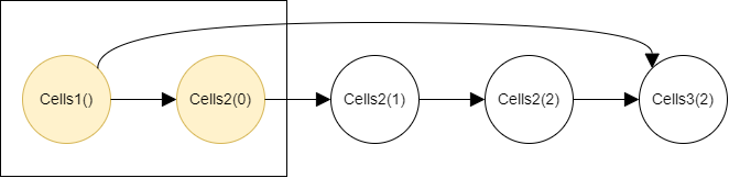
Because there is no node whose value can be cleared, the second step begins and the nodes in the second step are calculated.
And the 2 calculated nodes and the 2 value-pasted nodes from the previous step are checked whether their values should be pasted or cleared:
-
The value of
Cells2(2)is pasted because the node has an edge going out of the second step and referenced by theCells3(2)in the next third step. -
The value of
Cells2(1)is cleared because the node has an edge going out, but its destination isCells2(2), which is within the current second step. -
The value of
Cells2(0)is cleared because the node has an edge going out, but its destination isCells2(1), which is within the current second step. -
The value of
Cells1()is kept because the node has an edge going beyond the current second step and referenced by theCells3(2)in the next third step.
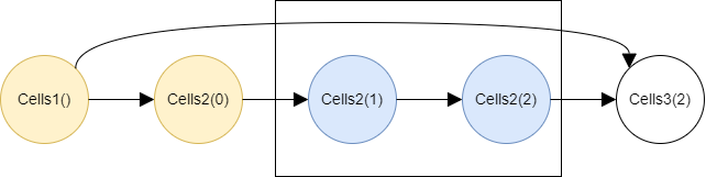
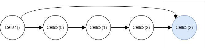
Then the third step begin and the target Cells3(3) node is calculated.
The target’s value is pasted and the value of all other nodes are cleared.
Since this is an illustrative example, the values of 4 out of 5 nodes are held at most at a certain point, so the memory-saving impact looks small, but in reality they are hundreds of thousands of nodes are involved, so the benefit is material.
The new feature design
In order for the mechanism above to work, the dependency graph of calculation nodes must be known first. modelx determines the dependency upon execution, so the mechanism requires 2 runs, one for generating the graph and a list of actions and the other for getting the target’s result. The first run should be carried out with a reduced set of model points.
The current design of the mechanism
introduces two new methods of the Model class. (They may be renamed by their official introduction)
generate_actionsexecute_actions
The generate_actions method is for generating the action list.
Each element in the lis is a list, whose first element is either
"calc", "paste" or "clear", and whose second element is a list
of nodes that the action denoted by the first element applies to.
"calc", "paste" and "clear" appear always in this order and together they compose
a single step.
In the case of the example above, the action list looks like below:
[['calc', [Model1.Space1.Cells1(), Model1.Space1.Cells2(x=0)]],
 ['paste', [Model1.Space1.Cells2(x=0), Model1.Space1.Cells1()]],
 ['clear', []],
 ['calc', [Model1.Space1.Cells2(x=1), Model1.Space1.Cells2(x=2)]],
 ['paste', [Model1.Space1.Cells2(x=2)]],
 ['clear', [Model1.Space1.Cells2(x=1), Model1.Space1.Cells2(x=0)]],
 ['calc', [Model1.Space1.Cells3(x=2)]],
 ['paste', [Model1.Space1.Cells3(x=2)]],
 ['clear', [Model1.Space1.Cells1(), Model1.Space1.Cells2(x=2)]]]
The execute_actions method takes this list as an argument, and
carry out the second run following the action list.
Testing with the lifelib model
Now let’s see how this works with CashValue_ME.
Our target node is result_pv(). For generating the action list, we use the default 4 model points.
>>> model = mx.read_model('CashValue_ME')

>>> model.Projection.model_point_table
         spec_id  age_at_entry sex  ...  premium_pp  av_pp_init  accum_prem_init_pp
poind_id                            ...
1              A            20   M  ...      500000           0                   0
2              B            50   M  ...      500000           0                   0
3              C            20   M  ...        1000           0                   0
4              D            50   M  ...        1000           0                   0

[4 rows x 10 columns]

>>> actions = model.generate_actions([model.Projection.result_pv.node()])
UserWarning: call stack trace activated
UserWarning: call stack trace deactivated
Using the generated action list, let’s calculate result_pv() for the 100K model points.
>>> df = pd.read_excel('model_point_table_100K.xlsx', index_col=0)

>>> df
          spec_id  age_at_entry sex  ...  duration_mth  premium_pp  av_pp_init
policy_id                            ...
1               B            47   M  ...             0      804000           0
2               C            29   F  ...             0         900           0
3               B            51   F  ...             0      409000           0
4               A            32   M  ...             0      128000           0
5               B            28   M  ...             0      698000           0
          ...           ...  ..  ...           ...         ...         ...
99996           C            21   M  ...             0         300           0
99997           A            24   F  ...             0      928000           0
99998           A            46   F  ...             0      662000           0
99999           C            46   M  ...             0        1500           0
100000          D            35   M  ...             0        1200           0

[100000 rows x 9 columns]

>>> model.Projection.model_point_table = df

>>> model.execute_actions(actions)

>>> model.Projection.result_pv()
               Premiums         Death  ...  Change in AV  Net Cashflow
policy_id                              ...
1          4.984800e+07  1.279624e+06  ...  8.705435e+06  4.656817e+06
2          5.992953e+06  1.871726e+06  ...  2.093446e+06  1.213795e+06
3          1.799600e+07  2.118581e+05  ...  1.495734e+06  4.955837e+05
4          1.088000e+07  7.187407e+04  ...  1.308987e+06  6.982380e+05
5          1.116800e+07  9.580780e+04  ...  1.970349e+06  1.031167e+06
                 ...           ...  ...           ...           ...
99996      1.659954e+06  3.911611e+05  ...  6.756107e+05  9.695319e+04
99997      7.145600e+07  3.429920e+05  ...  8.608484e+06  9.558065e+06
99998      4.435400e+07  6.358990e+05  ...  5.306157e+06  5.714497e+06
99999      6.186197e+06  3.169811e+06  ...  1.435512e+06  1.195544e+06
100000     1.878978e+07  7.463046e+06  ...  6.067500e+06  3.252222e+06
[100000 rows x 9 columns]
Here’s how how memory consumption increases during the run.

The maximum additional consumption is less then 9 GB, 30% of the original run, and the run time is actually shorter than the original run.