RECENT POSTS
- Introducing modelx-cython: Boosting modelx with Cython Compilation
- A First Look at Python in Excel
- Enhanced Speed for Exported lifelib Models
- New Feature: Export Models as Self-contained Python Packages
- Why you should use modelx
- New MxDataView in spyder-modelx v0.13.0
- Building an object-oriented model with modelx
- Why dynamic ALM models are slow
- Running a heavy model while saving memory
- Running modelx in parallel using ipyparallel
- All posts ...
Building an object-oriented model with modelx
May 5, 2022
Multiple objects of similar types tend to have common definitions of logic and data. Modeling these objects manually one by one is not a good idea, because you would end up having multiple copies of the same definitions, which are hard to maintain and error prone.
modelx supports an inheritance mechanism, which enables you to define the parts common to the multiple objects only once as part of a base object, and model each object by inheriting from the base object and defining only the parts unique to the object. By making full use of inheritance, you can organize the multiple objects sharing similar features into inheritance trees, minimizing duplicated formulas and keeping your model organized and transparent while maintaining the model’s integrity.
Inheritance in object-oriented programming
You may have heard about object-oriented programming (OOP). OOP is a programming paradigm, and most modern programming languages, such as Python and C++, support OOP. Such languages include powerful mechanisms, such as inheritance, for elegantly modeling complex objects. Inheritance in the OOP languages greatly enhances code reusability and extensibility.
modelx is inspired by OOP, and implements an inheritance mechanism similar to that of OOP. However, while most popular object-oriented programming languages use class-based inheritance, modelx uses prototype-bases inheritance.
Python for example uses class-based inheritance. Python lets you define classes and objects are instances of the classes. Inheritance relationships in Python are defined in terms of classes.
In modelx, there is no class equivalent, and inheritance relationships are defined between Space objects. A space object inherits from another space object, in order to use the other object as a prototype.
How Inheritance works in modelx
An inheritance relationship is established when you define a space(let’s name it A)
as a base space of another space(let’s name it B).
In this case, A is called a base space of B, and
B is called a sub space of A.
When B inherits from A, copies of all the cells, references and spaces contained in A are automatically created in B. This automatic copying is called deriving.
For example, let A have a child cells foo and a child reference bar.
As the figure shows, another set of foo and bar are derived in B.
The lines between A and B with a hollow triangle arrowhead on the side of A
indicates that B inherits from A.
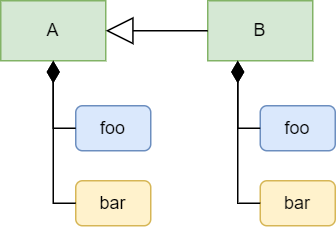
Initially, the formula of foo and the value of bar in B
are copied from those in A, but you can update foo’s formula and bar’s value
in B. This act of updating derived objects are called overriding.
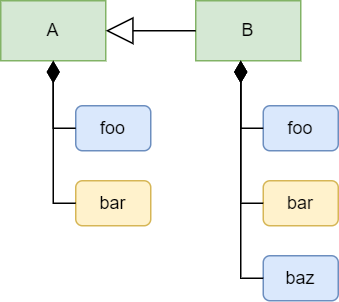
You can also add a new child object in B, for example a new cells named baz.
Adjustable-mortgage Example
Let’s learn how to implement inheritance by modeling a simple financial product.
In the modelx tutorial, a simple fixed-rate mortgage loan is modeled as the Fixed space.
Let’s say we also want to model an adjustable-rate mortgage loan.
For simplicity, we assume the adjustable-rate mortgage has the same loan term and principal as the fixed-rate mortgage’s.
Let the loan term be 10, and the principal be 100,000 in this example.
During the first 5 years, the interest rate of the adjustable mortgage is fixed at 2%, but from the 6th year the interest rate is updated every year till the end of the loan period. Let’s assume the interest rate is expected as follows:
| Year | 1 | 2 | 3 | 4 | 5 | 6 | 7 | 8 | 9 | 10 |
|---|---|---|---|---|---|---|---|---|---|---|
| Interest Rate | 2% | 2% | 2% | 2% | 2% | 4% | 5% | 6% | 5% | 4% |
Note that the interest rate applicable after the first 5 years is not known at the inception of the loan, because the rate is not fixed in advance. So the interest rate table above is an assumption or a scenario if we are modeling a loan to be paid off at a future point in time.
We want to model the adjustable mortgage as the Adjustable space.
Since Fixed and Adjustable are both mortgages and expected to have some shared
definitions of formulas and values, we can make use of inheritance.
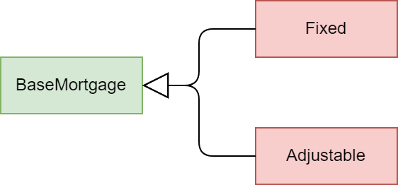
we create a base space, BaseMortgage, and define cells and references
common to Fixed and Adjustable in BaseMortgage.
Fixed and Adjustable inherit from BaseMortgage, and we override
some of the derived objects inherited from BaseMortgage to reflect their own features. The diagram below depicts the relationship of the spaces.
To identify the commonality between the two types of mortgages, let’s review the contents of Fixed from the earlier example one by one,
and think about whether and how they should be updated.
-
Termis an integer representing the length of the loan term in years. We’ve assumed above that the fixed and adjustable mortgages have the same term. -
Principalrepresents the initial loan balance and is given as an input. We’ve assumed above that the principals of the fixed and adjustable mortgages are the same amount. -
Rateis a constant interest rate that applies through the lifetime of the fixed mortgage. Since the interest rate onAdjustableis adjusted periodically,RateforAdjustableshould have a different definition from that ofFixed. The adjustable interest rate can be defined as adictindexed with loan duration. -
Paymentrepresents the amount of a payment to be made regularly to repay the loan. In the case ofFixed,Paymentis defined as the constant amount calculated fromPrincipal,Term, andRate.PaymentforAdjustableneeds to be time-dependent, because it is recalculated periodically in response to changes in the interest rate. We will redefine the formula ofPaymentto make it time-dependent and applicable to bothFixedandAdjustable. -
Instead of directly referring to
RatefromPayment, it’s better to refer toRatefromPaymentindirectly through a new cells with a time index, because the fixed and adjustable rate can be referenced with the time index in the same fashion. Let’s name the cellsIntRate. -
Balanceis indexed with the time indext, and represents the remaining balance of the loan at timet. The formula ofBalancecalculates the loan balance at timetrecursively from the previous balance. The initial balance is input fromPrincipalandRateis referenced for interest accretion. By replacingRatewithIntRate(t), the formula becomes common betweenFixedandAdjustable.
The tables below summarizes how the contents of each space should be defined.
| Contents | BaseMortgage |
Fixed |
Adjustable |
|---|---|---|---|
Term |
10 | Inherited from BaseMortgage |
Inherited from BaseMortgage |
Principal |
100000 | Inherited from BaseMortgage |
Inherited from BaseMortgage |
Rate |
To be defined | 0.03 | a dict object |
Payment(t) |
Shared formula | Inherited from BaseMortgage |
Inherited from BaseMortgage |
IntRate(t) |
To be defined | Unique formula | Unique formula |
Balance(t) |
Shared formula | Inherited from BaseMortgage |
Inherited from BaseMortgage |
You may have noticed that instead of creating BaseMortgage,
it is possible to model Adjustable by inheriting from Fixed.
Although it’s technically possible, it’s not a good design, because
the adjustable mortgage is not a special form of the fixed mortgage.
Good practice is to make sure that an inheritance relationship should
always represent “is a” relationship.
Modeling Inheritance
We start from the Mortgage model from the earlier example, but you may also start from scratch if you prefer.
>>> import modelx as mx

>>> model = mx.read_model(`Mortgage`)
Let’s use the Fixed space as the base space. Rename it BaseMortgage
>>> model.Fixed.rename('BaseMortgage')

>>> model.BaseMortgage
<UserSpace Mortgage.BaseMortgage>
Now set 10 to Term, which is a constant shared between the sub spaces.
>>> model.BaseMortgage.Term = 10
Now let’s create Fixed under the model by inheriting from BaseMortgage. You can do so by passing BaseMortgage to the bases parameter of the model’s new_space method.
>>> model.new_space('Fixed', bases=model.BaseMortgage)
In the same way, create Adjustable by inheriting from BaseMortgage.
>>> model.new_space('Adjustable', bases=model.BaseMortgage)
You can also define an inheritance relationship between existing spaces
using the add_bases method. Alternatively to calling the new_space
with the bases parameter, you could also create Fixed and Adjustable
by calling new_space without bases, and later calling
add_bases on Fixed and Adjustable to set BaseMortgage as their
base space:
>>> model.new_space('Fixed')

>>> model.new_space('Adjustable')

>>> model.Fixed.add_bases(model.Mortgage)

>>> model.Adjustable.add_bases(model.Mortgage)
Next, we set the interest rates by duration for Adjustable as a dict.
Note that the index starts from 0, so the key for the Nth rate is (N-1).
>>> model.Adjustable.Rate = {
...     0: 0.02,
...     1: 0.02,
...     2: 0.02,
...     3: 0.02,
...     4: 0.02,
...     5: 0.04,
...     6: 0.05,
...     7: 0.06,
...     8: 0.05,
...     9: 0.04
... }
You may also assign 0.03 to Rate in Fixed, although the value is inherited.
>>> model.Fixed.Rate = 0.03
To refer to Rate in the same manner in both Fixed and Adjustable,
we create a cells IntRate indexed with t.
First we create IntRate in BaseMortgage and define its formula to raise a NotImplementedError to indicate that it needs to be defined in the sub spaces.
There are a few ways to define the formula of IntRate.
Here we define it by first defining a Python function and then assigning it
to InitRate’s formula.
>>> IntRate = model.BaseMortgage.new_cells('IntRate')

>>> def temp(t): # the name of the function can be anything.
        raise NoteImplementedError

>>> IntRate.formula = temp

>>> IntRate.formula
def IntRate(t):
    raise NoteImplementedError
Then override IntRate in Fixed and Adjustable to refer to their own Rate.
>>> model.Fixed.IntRate.formula = lambda t: Rate

>>> model.Adjustable.IntRate.formula = lambda t: Rate[t]

>>> model.Adjustable.IntRate[5]
0.04
Next, we are going to define Payment in BaseMortgage so that the definition of Payment in the base space can be inherited and used both in Fixed and Adjustable
without change.
The formula before update should look like below in BaseMortgage because
we developed it from Fixed form the earlier example.
def Payment():
    return Principal * Rate * (1+Rate)**Term / ((1+Rate)**Term - 1)
The formula above exactly represents the math expression below, which is a known formula to calculate the amount of level annual payments to pay off in Term years
a debt with interest accruing at Rate a year.
To make the formula applicable to Adjustable, we need to apply the following changes.
- Parameterize
Paymentwitht - Replace
RatewithIntRate(t-1) - Replace
PrincipalwithBalance(t-1) - Replace
TermwithTerm - t + 1
The expression now looks like below:
Balance(t-1) * IntRate(t-1) * (1 + IntRate(t-1))** (Term - t + 1) / ((1 + IntRate(t-1))** (Term - t + 1) - 1)
The corresponding math expression is as follows:
\[Payment(t) = Balance(t-1)\cdot\frac{IntRate(t)(1+IntRate(t))^{Term-t+1}}{(1+IntRate(t))^{Term-t+1}-1}\]You may wonder why Payment(t) refer to Balance(t-1) and IntRate(t-1),
instead of Balance(t) and IntRate(t).
You may also wonder why the remaining period is not Term - t but Term - t + 1.
The figure below illustrates how Payment(6) is calculated.
Payment(6) is calculated at t=5 such that paying the amount for the rest of
the loan term (5 years) would pays off Balance(5) with interest accruing at IntRate(5),
assuming that IntRate(5) would apply for the rest of the loan period.

In reality, the interest rate is updated annually, so one year later at t=6, the IntRate(6) may be different from IntRate(5). In that case, Payment(7) is updated
such that the updated amount would pays off Balance(6) with interest
accruing at IntRate(6) for the rest of the loan term.

Note the Payment formula above is also valid for Fixed, because
the formula Payment returns the same value for t during the loan period if
the interest rate does not change. So we define Payment in BaseMortgage.
The code below update Payment in BaseMortgage.
r and u are defined to make the expression compact.
>>> def temp(t):
...     r = IntRate(t-1)
...     u = Term - t + 1
...     return Balance(t-1) * r * (1 + r)**u / ((1 + r)**u - 1)

>>> model.BaseMort.Payment.formula = temp
We need to update one more cells. Balance is defined in BaseMortgage as follows.
>>> model.Mortgage.Balance.formula
def Balance(t):

    if t > 0:
        return Balance(t-1) * (1+Rate) - Payment
    else:
        return Principal
The formula should refer to IntRate(t-1) and Payment(t) instead of Rate
and Payment respectively:
>>> def temp(t):
...     if t > 0:
...         return Balance(t-1) * (1 + IntRate(t-1)) - Payment(t)
...     else:
...         return Principal

>>> model.BaseMortgage.Balance.formula = temp
Checking the results
Now that we have completed making all the necessary changes,
let’s check the results.
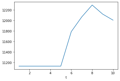
Below the adjustable payments are output as a dict.
As expected, the payments increase after the first 5 years
because the interest rate at t=5 is higher than before.
The payments then vary every year, reflecting the changes in the interest rate.
>>> {t: model.Adjustable.Payment(t) for t in range(1 ,11)}
{1: 11132.652786531637,
 2: 11132.65278653164,
 3: 11132.652786531638,
 4: 11132.652786531644,
 5: 11132.65278653164,
 6: 11786.927741021387,
 7: 12065.96444749335,
 8: 12292.72989621633,
 9: 12120.72411143264,
 10: 12005.288643704713}
>>> model.Adjustable.Payment.series.plot()
To compare against the adjustable payments,
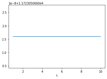
let’s also output and plot the fixed payments.
As you see below, the fixed payments are constant
throughout the loan period, even though the payments
are recalculated every year by the formula shared with Adjustable.
>>> {t: model.Fixed.Payment(t) for t in range(1 ,11)}
{1: 11723.050660515952,
 2: 11723.050660515952,
 3: 11723.050660515953,
 4: 11723.050660515959,
 5: 11723.05066051596,
 6: 11723.050660515968,
 7: 11723.05066051596,
 8: 11723.050660515977,
 9: 11723.05066051599,
 10: 11723.05066051596}
>>> model.Fixed.Payment.series.plot()
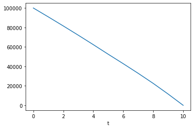
Below is the output of Adjustable.Balance.
You can see that the balance is actually paid off at t=0.
>>> {t: model.Adjustable.Balance(t) for t in range(0 ,11)}
{0: 100000,
 1: 90867.34721346837,
 2: 81552.0413712061,
 3: 72050.42941209857,
 4: 62358.78521380889,
 5: 52473.30813155344,
 6: 42785.31271579419,
 7: 32858.613904090555,
 8: 22537.40084211966,
 9: 11543.546772793003,
 10: 1.0913936421275139e-11}
>>> model.Adjustable.Balance.series.plot()
