New Feature: Export Models as Self-contained Python Packages

Overview

The latest release of modelx, v0.22.0, introduces an exciting new feature that enables users to export modelx models as self-contained Python packages.

This export feature is still in its experimental stage, and certain limitations apply as detailed further in this post. However, it has proven effective for practical models, requiring little to no manual modifications. Furthermore, these limitations will be addressed in upcoming modelx versions.

Motivation

The integration of the export feature to modelx offers two significant advantages. Firstly, exported models run faster than their original versions. Secondly, the exported models function as standalone Python packages, independent of modelx. They are composed in plain Python, providing users with increased transparency and abundant opportunities to merge these exported models with other tools in the Python ecosystem.

Let’s delve deeper into these benefits. modelx allows you to efficiently construct complex financial models interactively through the IPython interpreter or Spyder IDE. It achieves this by offering sophisticated types like Model, UserSpace, and Cells, which you can utilize to create objects and define your unique logic. By managing these objects, modelx enables you to define mathematical formulas as Python functions, executing and reusing them with various parameter sets. If you were to create the same model in plain Python, you’d need to implement these formulas as class methods to achieve a similar instantiation mechanism. To reference other methods and instance variables within a method, names must be prefixed by self., making the mathematical expressions more verbose and less readable. modelx also offers a host of other features like parameterization, dependency tracing, inheritance, and error reporting.

While these functionalities are undeniably beneficial, they do come with certain trade-offs. For one, modelx can introduce some overhead during model execution, as a lot occurs behind the scenes to ensure these rich features function correctly.

Moreover, although modelx models are stored in plain-text files, these files are pseudo-Python modules and are not directly executable by the Python interpreter. Instead, these files can only be interpreted by modelx to bring to life live objects within Python sessions.

The export feature aims to address these modelx limitations. It allows you to transform a live modelx model into a Python package. This generated package is self-contained and operates independently of modelx. The package comprises modules that contain Python class definitions for the model, and for each space within the model. Cells and references are implemented as class methods and attributes. The export feature automatically detects the names of methods and member variables in the method definitions, prefixing them with self.. Furthermore, the package includes files storing data and metadata utilized in the model.

Upon importing the package, an instance of the model class is created. This instance can be accessed as mx_model, or under the name of the original model within the package’s namespace. Though the exported model lacks certain features that the original modelx model possesses for live editing and inspection, it still produces results consistent with the original modelx model.

Example

Let’s examine the export feature with a simple case study. Suppose we wish to price call options on an equity asset using the Black-Scholes formula for different combinations of the strike price (K) and volatility (sigma). The code snippet below constructs a modelx model for this task.

import modelx as mx
import math
from scipy import stats
import itertools


model = mx.new_model('Options')
bs = model.new_space('BlackScholes')


bs.math = math
bs.stats = stats
bs.S0 = 100     # Underlying asset price
bs.T = 3        # Time to expiration in years
bs.K = 110      # Strike price
bs.r = 0.05     # Risk-free interest rate
bs.sigma = 0.2  # Volatility


@mx.defcells
def call_opt():
    d1 = (math.log(S0 / K) + (r + 0.5 * sigma ** 2) * T) / (sigma * math.sqrt(T))
    d2 = d1 - sigma * math.sqrt(T)
    return S0 * stats.norm.cdf(d1) - K * math.exp(-r * T) * stats.norm.cdf(d2)


bs.parameters = ('K', 'sigma')
summary = model.new_space('Summary')
summary.itertools = itertools
summary.bs = bs


@mx.defcells
def result():
    params = itertools.product([100, 110], [0.2, 0.3])
    return [{'K': k, 'sigma': s, 'price': bs[k, s].call_opt()} for k, s in params]

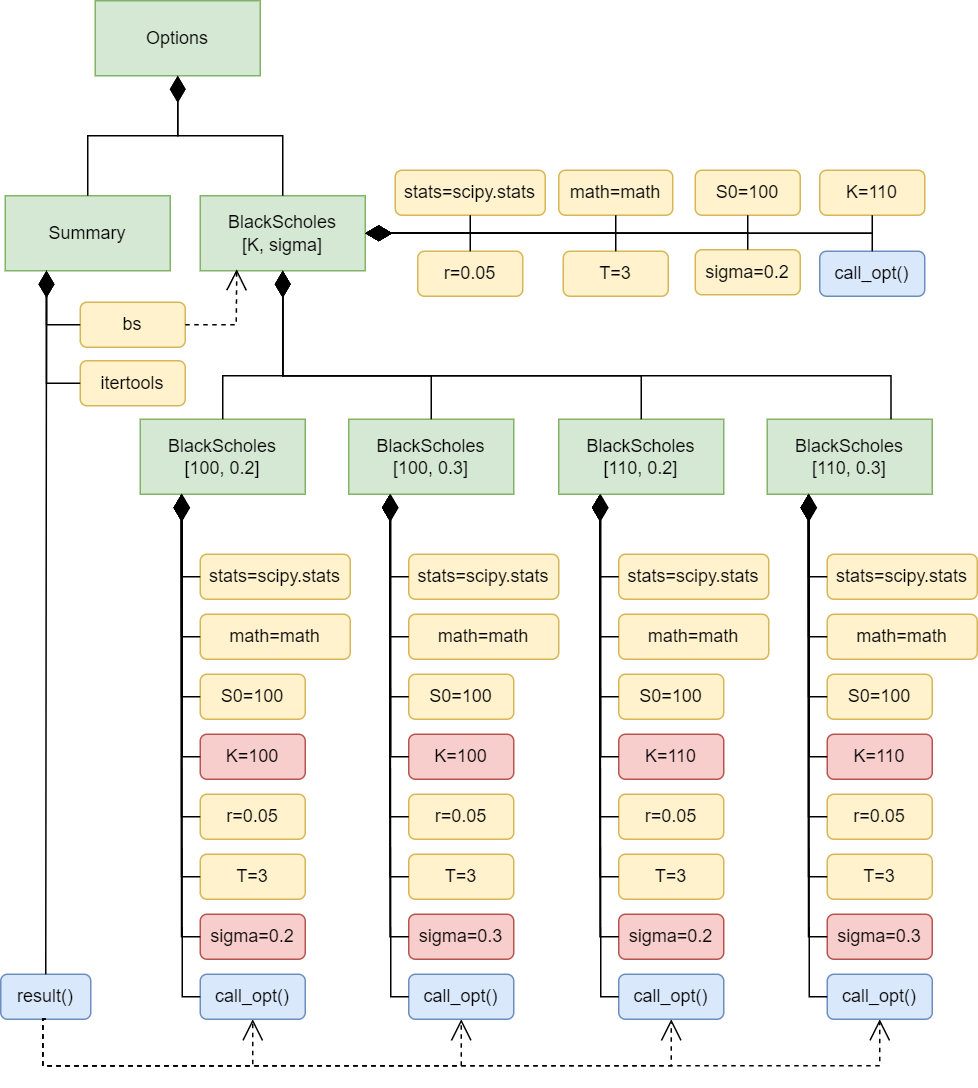
The above code first constructs a modelx Model object, Options, and assigns it to model in the global namespace. Within this model, a space called BlackScholes is created and assigned to bs for ease of access. This space receives the necessary parameters for the Black-Scholes formula, such as S0, T, K, r, and sigma, along with modules like math and scipy.stats.

The call_opt function, decorated with @mx.defcells, defines a Cells object. This function, when called, calculates the call option value for the provided parameter values.

>>> call_opt()
16.210871364283975

Since we’re interested in option values for various combinations of K and sigma, we parameterize the BlackScholes space with these variables. This allows the space to dynamically clone itself when called or subscripted with values for K and sigma. The code below retrieves the option values for K equal to 110 and sigma equal to 30%.

>>> bs[110, 0.3].call_opt()
22.722279541172703

Next, we create a new space named Summary, adjacent to BlackScholes. This space is designated for summarizing the results of the option values and providing the summary as a dict, keyed by the pair of the values of K and sigma. The BlackScholes space is referenced as bs within the Summary space, and the result Cells object is defined by a function definition. The itertools standard library is also assigned within the Summary space, which is used in the result formula to generate all possible combinations of 100 and 110 for K, and 20% and 30% for sigma.

>>> result()
[{'K': 100, 'sigma': 0.2, 'price': 20.924360952895213},
 {'K': 100, 'sigma': 0.3, 'price': 26.805483596641537},
 {'K': 110, 'sigma': 0.2, 'price': 16.210871364283975},
 {'K': 110, 'sigma': 0.3, 'price': 22.722279541172703}]

The diagram below depicts the structure of the Options model.

Now, let’s test the export feature. You can use the new API function export_model or the export method on Model to achieve this. The following code exports the Options model to the Options_nomx package in the current directory.

>>> model.export('Options_nomx')

When you import the package, it creates an instance of the exported Python model as mx_model or Options, both referring to the same object.

>>> from Options_nomx import mx_model, Options

>>> mx_model is Options
True

You can interact with the self-contained model in the same manner as with the original modelx model.

>>> mx_model.BlackScholes.call_opt()
16.210871364283975

>>> mx_model.BlackScholes[110, 0.3].call_opt()
22.722279541172703

>>> mx_model.Summary.result()
[{'K': 100, 'sigma': 0.2, 'price': 20.924360952895213},
 {'K': 100, 'sigma': 0.3, 'price': 26.805483596641537},
 {'K': 110, 'sigma': 0.2, 'price': 16.210871364283975},
 {'K': 110, 'sigma': 0.3, 'price': 22.722279541172703}]

The Contents of the Self-Contained Python Package

The Options_nomx package, generated by our previous example, includes the following files:

• __init__.py: This is the initialization file for the Options_nomx package. It imports the names mx_model and Options from _mx_model.py into the namespace of Options_nomx.
• _mx_sys.py: This file defines base classes along with other classes and global variables common to all exported models.
• _mx_model.py: This file defines the _c_Options class and its instance, the Options model.
• _mx_classes.py: This file defines the _c_BlackScholes and _c_Summary classes for the space objects within the Options model.

The core logic is contained within _mx_class.py. In this file, you can confirm that call_opt and result are defined as methods, with all relevant names in their definitions appropriately prefixed by self..

Note that additional files and directories may also be generated based on the specific details of your model. For instance, if your model contains a PandasData object, a corresponding data file for that object (either an Excel file or a CSV file) would be generated, along with a _mx_io.py file containing the metadata of the pandas object.

Furthermore, if your model contains a reference bound to a pickle-able object, the pickled data would be stored in the _mx_pickled file. In the case where the spaces within your model contain nested spaces, subdirectories would be created within the package. The contents of these nested spaces would be defined in files within these subdirectories.

Limitations

While the feature works effectively for most models, it’s still in an experimental phase. Hence, there are a few limitations:

• Relative References in ItemSpaces: Currently, relative references within an ItemSpace aren’t supported. This means that all references within an ItemSpace are bound to the same objects that their base references point to. This is relevant if your model has nested spaces, where one space refers to another in the ItemSpaces. Rest assured, we plan to address this limitation in upcoming modelx releases.

• Coercion of Parameterless Cells: In modelx, a Cells object without parameters is coerced to its value when used as an operand of arithmetic operators (such as +, -, *, /). However, this coercion is not implemented in exported models. Rather than implementing this in exported models, the plan is to deprecate this behavior in future modelx releases. This coercion introduces overhead and potentially errors, so users should be advised to remove the coercion and ensure that such Cells are explicitly called using () in the original model’s formulas.

• Objects Associated with IOSpec: Support for objects associated with IOSpec, other than PandasData (such as ExcelRange and ModuleData), is not yet provided. this limitation will be addressed in future modelx releases.

Next Steps

The immediate next step for this feature is, naturally, to address the existing limitations. Alongside this, more tests will be conducted using a wide variety of modelx models. A performance comparison between the original modelx models and their exported counterparts is certain to be illuminating.

Viewing this from a long-term perspective, the export feature brings us one step closer to implementing a conversion feature that would allow modelx models to be transformed into statically-typed, compiled models. This would be achieved by utilizing Python’s type hints and Cython. The future of modelx is thrilling, with the integration of this export feature opening up fresh opportunities to leverage the power of Python for diverse modeling needs.