Why dynamic ALM models are slow

In this post, we discuss dynamic ALM models used in life actuarial practices. Especially, we discuss why it’s so hard to develop efficient dynamic ALM models from computing technology perspectives.

What is a dynamic ALM model?

An ALM model projects the cashflows of a portfolio of insurance policies and assets backing the policies.

Not all ALM models have to be dynamic. An ALM model has to be dynamic when the cashflows of the modeled insurance policies depend on the investment return on the portfolio of the backing assets. An example of such dependency is a feature that sum assured increases depending on the investment performance. Another example is a dynamic lapse assumption, which reflects the dependency of policyholder’s behavior on the investment performance.

Note that you don’t need a dynamic ALM model (thus you only need a static model) when the cashflows of the modeled insurance products do not depend on the investment return. Most protection products without saving features don’t required dynamic models.

You also do not need a dynamic ALM model for variable annuities (VA). Since each VA policy has its own account value, the investment return for each individual policy can be calculated separately. So the cashflows of the policy do not depend on the investment return on the portfolio of the backing assets, which makes the ALM model much simpler.

Even when you model index-linked products or universal life products with dynamic lapse assumptions, dynamic ALM models are not necessary if the investment return is a function only of indices observed in the market, and not dependent on the performance of the asset portfolio backing the policies.

How a dynamic ALM model works

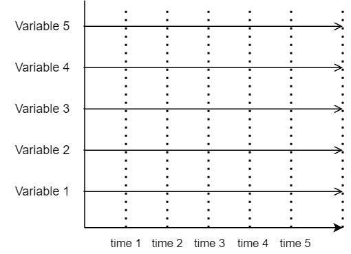
The liability model of a policy (a single model point) is a set of variables most of which are functions of time. The variables represent projection items, such as various cashflows and changes in the number of in-force policies. The figure below represents the liability model, and Variable 1, 2, 3… could be, for example, premium income, death benefits, number of in-force policies, etc.

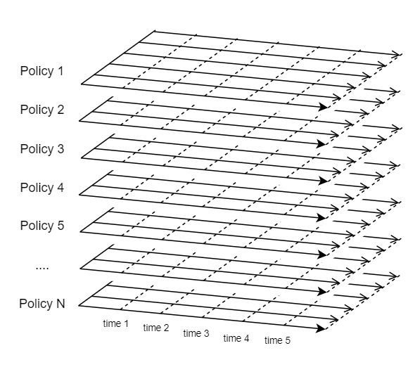
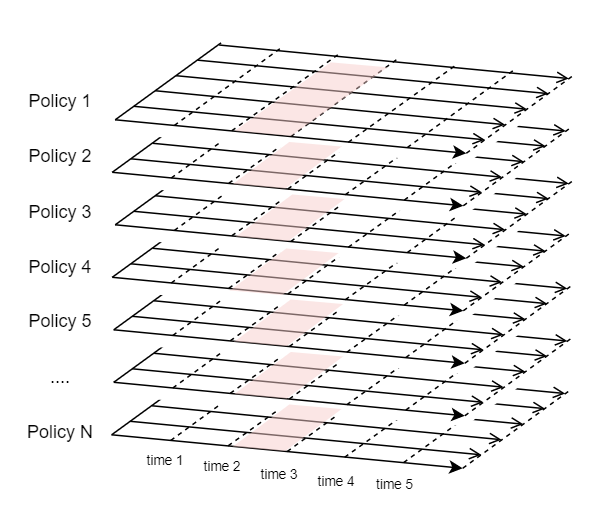
The liability model of the entire liability portfolio calculates the total cashflows, by calculating the cashflows of individual model points one by one, iterating over the portfolio and summing up the cashflows of individual model points. The figure below represents the liability model of a liability portfolio. Each surface in the figure represents one model point in the portfolio.

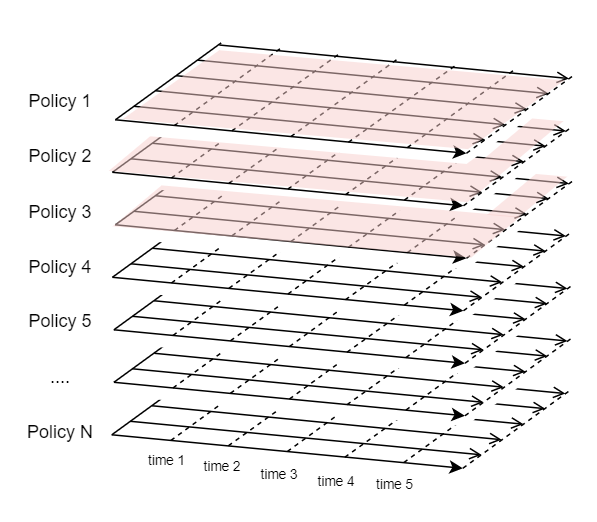
In case of a static model, you can model cashflows of insurance policies separately from the asset cashflows. The figure below illustrates the calculation order of a static model. As indicated by the highlighted surfaces from the top, first the variables of Policy 1 are calculated for all time periods, and the variables of Policy 2 are calculated for all time periods, and so on.

The portfolio in reality is composed of as many as 100 thousands or more policies, and the number of variables can be hundreds or more. So if you keep all the calculated values of all the variables for all the policies in the portfolio, the data size on the memory would become huge and eventually exceed the size of the physical memory equipped in your computer.

Luckily, in case of a statice model, you don’t need to keep the calculated values of individual model points, because each model point can be calculated separately, i.e. to calculate variables for one model point, you don’t need the results of other model points. And unless you are debugging the model, you’are only interested in the total values of certain variables, so you only need to have one set of the selected variables for storing the total values, and after each model point is processed, you can add the model point’s results to the total variables, and clear the results of the model point.

However, dynamic ALM models don’t carry out calculations in the same order as static models. The figure below illustrates the order of liability calculations in case of a dynamic ALM model.

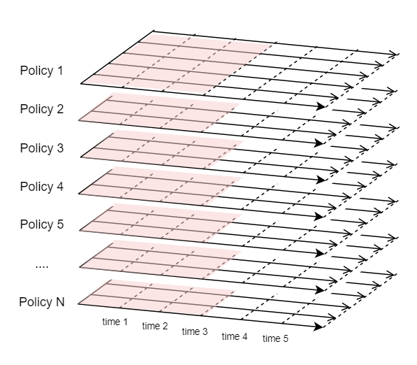
First, the values of variables for the first time period (time 0 through time 1) for all the policies are calculated. Then the total liability cashflows for the first period are fed into the asset model, and the investment return for the 1st period is received from the asset model and the values of the variables for the 2nd period are calculated for all the policies in the liability portfolio. Unlike a static model, a dynamic ALM model cannot process policies one after another. You cannot clear the values of other model points calculated before each policy is processed.

This is why a dynamic model tends to consume a lot of memory and eventually runs slow. But as you may have noticed, there is still a way to reduce the memory consumption. To calculate the values of variables for the 4th period (time 3 through time 4) for example, you would only need the values of variables for the 3rd period, and the values of the 1st and 2nd periods can be cleared, as the figure below illustrates.

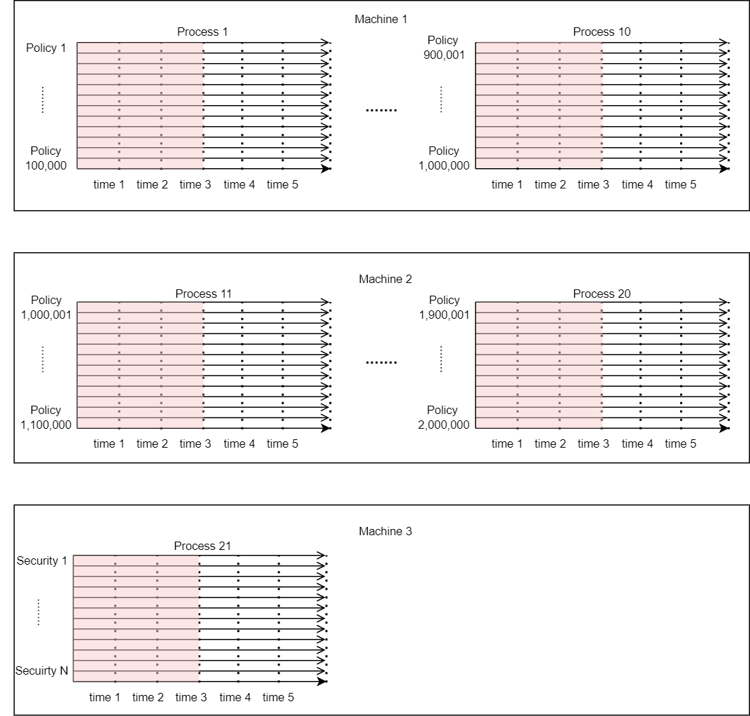
The calculation order of dynamic ALM models introduces another complexity of concurrency when the calculations of the liability portfolio are distributed across multiple processes on multiple machines.

It is often then case that a liability portfolio contains a large number of policies and the liability calculations are distributed across multiple processes on multiple machines. Let’s say the liability portfolio has 2 million policies. The policies could be grouped into 20 groups of policies, each of which contains 100,000 policies. Group 1 through Group 10 could be processed in parallel on Machine 1, and Group 11 through 20 could be processed in parallel on Machine 2, and the asset model could be processed on Machine 3. As the figure below illustrates, all the 21 processes need to be processed synchronously in terms of the time axis. The synchronous processing involves stopping a process at a certain point and resuming it at another point. It also involves data transfer between the processes because the liability cashflows are aggregated and the investment return needs to be fed back from the asset process to each liability process.

Summary

A dynamic ALM model is needed when the cashflows of the modeled insurance policies depend on the investment return on the portfolio of the backing assets. A dynamic ALM model works differently from a static ALM model, and its calculation order introduces computational challenges, such as memory overload and synchronous processing. Understanding the mechanism helps you identify bottlenecks and solve performance issues of your dynamic ALM model.