RECENT POSTS
- Introducing modelx-cython: Boosting modelx with Cython Compilation
- A First Look at Python in Excel
- Enhanced Speed for Exported lifelib Models
- New Feature: Export Models as Self-contained Python Packages
- Why you should use modelx
- New MxDataView in spyder-modelx v0.13.0
- Building an object-oriented model with modelx
- Why dynamic ALM models are slow
- Running a heavy model while saving memory
- Running modelx in parallel using ipyparallel
- All posts ...
fastlife got faster
Jan 31, 2021 • Fumito Hamamura
In my previous post, I introduced a prototype of fastlife, a model that processes multiple model points in parallel, and mentioned a few ways to improve it. I further worked on the model and made it run faster. The updated model is attached below for your reference. I’m planning to add the fastlife project to lifelib soon based on this version of prototype with some further changes.
Speed Before and After
The previous model took about 21 seconds on my PC as I wrote previously. This time, I ran the same model on a new Python environment on the same PC. This time, the model took about 14 seconds. The table below compares the versions of Python and relevant packages between the new and old environment. I don’t know what relevant package contributed to the performance improvement.
| Package | Old ver. | New ver. |
|---|---|---|
| Python | 3.7.4 | 3.7.6 |
| pandas | 0.25.1 | 1.1.2 |
| numpy | 1.16.5 | 1.19.2 |
| networkx | 2.3 | 2.4 |
| openpyxl | 3.0.0 | 3.0.3 |
Then I updated the model by making changes to the model as explained in the next section. The updated model only took 6.4 seconds for the same run. The base set of model points contains 300 model points, 100 of which are 15-year term policies, 100 of which are whole life policies with varying issue ages and 100 of which are 10-year endowment policies. Because all the policies are processed in parallel, the projection period lasts till the end of the last whole life policy, although all the term and endowment policies don’t exist beyond their maturities.
Since the run time is so short, I increased the number of model points by 10 and 100 times, just by copying the original set of model points. The model took 46 seconds and 449 seconds respectively. The run time per model point improved from the 300 model point run to the 3000 model point run, and it remains at almost the same level between the 3000 model point run to 30000. This is understandable given that some formulas are evaluated only once regardless of the number of model points.
| Python Env. | Model | No. MPs | Time(sec.) |
|---|---|---|---|
| Old | simplelife | 300 | 31 |
| Old | Previous | 300 | 21 |
| New | Previous | 300 | 14 |
| New | Updated | 300 | 6.4 |
| New | Updated | 10 x 300 | 46 |
| New | Updated | 100 x 300 | 449 |
Model Optimization
The table below lists the 5 most time consuming Formulas from the previous model.
| Formula | No. calls | Duration(Sec.) |
|---|---|---|
fastlife.Projection.Assumptions.MortFactor(y) |
103 | 6.298937321 |
fastlife.Projection.Assumptions.SurrRate(y) |
103 | 6.012678623 |
fastlife.Projection.Policy.ReserveNLP_Rate(basis, t) |
104 | 5.720100403 |
fastlife.Projection.BaseMortRate(t) |
103 | 1.585314989 |
fastlife.Projection.BenefitTotal(t) |
103 | 0.213982344 |
The first 3 Formulas accounts for more than 70% of the total run time.
I couldn’t refine ReserveNLP_Rate, but I was able to refine
MortFactor and SurrRate, as well as many other parts of the model.
Let me explain how I refined MortFactor Formula for example.
For every value of y, a callback function get_factor was called,
and get_factor looked up in the assumption table the mortality factor ID
for each model point in PolicyData that best matched the 3 model point
attributes, product ID, policy type ID and generation ID.
>>> fastlife.Projection.Assumptions.MortFactor.formula
def MortFactor(y):
    """Mortality factor"""

    def get_factor(pol, y):

        key1, key2, key3 = pol['Product'], pol['PolicyType'], pol['Gen']
        table = AsmpLookup.match("MortFactor", key1, key2, key2).value

        if table is None:
            raise ValueError('MortFactor not found')

        result = AssumptionTables.get((table, y), None)

        if result is None:
            return MortFactor(y-1)[pol.name]
        else:
            return result


    return PolicyData.apply(lambda pol: get_factor(pol, y), axis=1)
The mortality factor ID for each model point does not change over time,
so it’s redundant to look for the ID at every y.
So I created another Cells, named MortFactorID and
factored out the logic for the mortality factor ID lookup from MortFactor,
and put the logic in MortFactorID.
>>> fastlife.Projection.Assumptions.MortFactorID.formula
def MortFactorID():
    """Mortality factor"""

    def get_factor(pol):

        key1, key2, key3 = pol['Product'], pol['PolicyType'], pol['Gen']
        table = AsmpLookup.match("MortFactor", key1, key2, key2).value

        if table is None:
            raise ValueError('MortFactor not found')

        return table

    return PolicyData.apply(lambda pol: get_factor(pol), axis=1)
>>> fastlife.Projection.Assumptions.MortFactor.formula
def MortFactor(y):
    """Mortality factor"""

    fac = MortFactorID().apply(lambda facid: AssumptionTables.get((facid, y), np.NaN))

    if y == 0 or not fac.isnull().any():
        return fac
    else:
        return fac.mask(fac.isnull(), MortFactor(y-1))
I refactored SurrRate formula similarly. Thanks to these refinements,
the execution times of MortFactor and SurrRate reduced significantly,
and they are not the top 2 time consuming formulas anymore.
| Formula | No. calls | Duration(sec.) |
|---|---|---|
fastlife.Projection.Policy.ReserveNLP_Rate(basis, t) |
104 | 2.628533602 |
fastlife.Projection.BaseMortRate(t) |
103 | 1.553189516 |
fastlife.Projection.Assumptions.MortFactor(y) |
103 | 0.221627712 |
fastlife.Projection.BenefitTotal(t) |
103 | 0.140694857 |
fastlife.Projection.ExpsTotal(t) |
103 | 0.124999762 |
fastlife.LifeTable['M', 0.03, 3].AnnDuenx(x, n, k, f) |
1755 | 0.109314919 |
fastlife.Projection.Assumptions.SurrRate(y) |
103 | 0.094744205 |
Multi-core utilization
In the previous post, I explained how it’s hard to make Python scripts multithreaded effectively due to the GIL issue, and mentioned modin as a possible solution, hoping that it would have some mechanism to solve the issue under the hood.
I tested and learned more about modin and its underlying
Python library, dask. Unfortunately, modin and dask don’t seem to
solve the issue out of the box.
In many formulas in fastlife, Series.apply method is used. The
method is for calling back a Python function to apply the function
to each element of the Series.
Since the callback function is interpreted by the Python interpreter,
calls to the callback function can only be processed serially
within the same process because of GIL.
Given the complexity of actuarial models in general,
it would be difficult to completely get rid of Series.apply.
I thought about translating callback functions to native code by using cython or numba, but that doesn’t seem to be realistic because the callbacks could reference high-level Python objects, such as Space and Cells defined in modelx.
I stopped pursuing multithreading approaches for now, and shifted my attention to multiprocessing.
A modelx user contributed sample code to execute modelx in a specified number of parallel processes. By applying some changes to the contributed code, it didn’t take much time to make modelx run in parallel in separate processes. I made the code available here for your reference. Using the code, I tested running modelx in different numbers of processes, from 1 to 10, giving each process the 3000 model points as I used before, and observed how the run time grew.
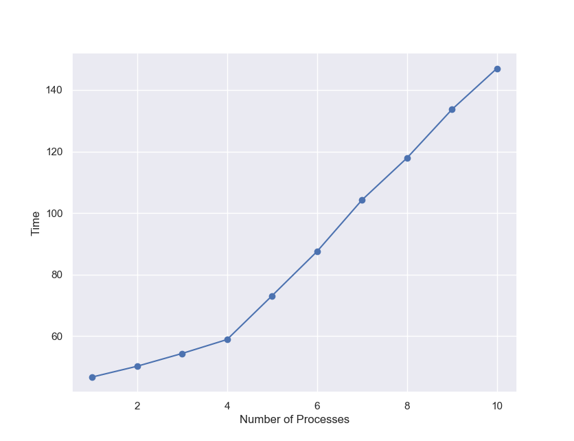
| No. Processes | Total No. Model Points | Time(sec.) |
|---|---|---|
| 1 | 3000 | 47 |
| 2 | 6000 | 50 |
| 3 | 9000 | 54 |
| 4 | 12000 | 59 |
| 5 | 15000 | 73 |
| 6 | 18000 | 88 |
| 7 | 21000 | 104 |
| 8 | 24000 | 118 |
| 9 | 27000 | 134 |
| 10 | 30000 | 147 |
Since my PC has 4 CPU cores, the execution time increases only by a 3-5 seconds up to the 4 processes run. From there, the time increases by about 15 seconds per process. Assuming that each additional process is evenly distributed across the 4 cores, 60 CPU seconds are spent on the additional run with the 3000 model points. This is understandable given that it takes 47 seconds for a single run and that there must be some overhead. Taking about 150 seconds for the 30000 model points also explains 30% overhead due to multiprocessing, which you can tell from the comparison against the single process run that took 450 seconds for the 30000 model points
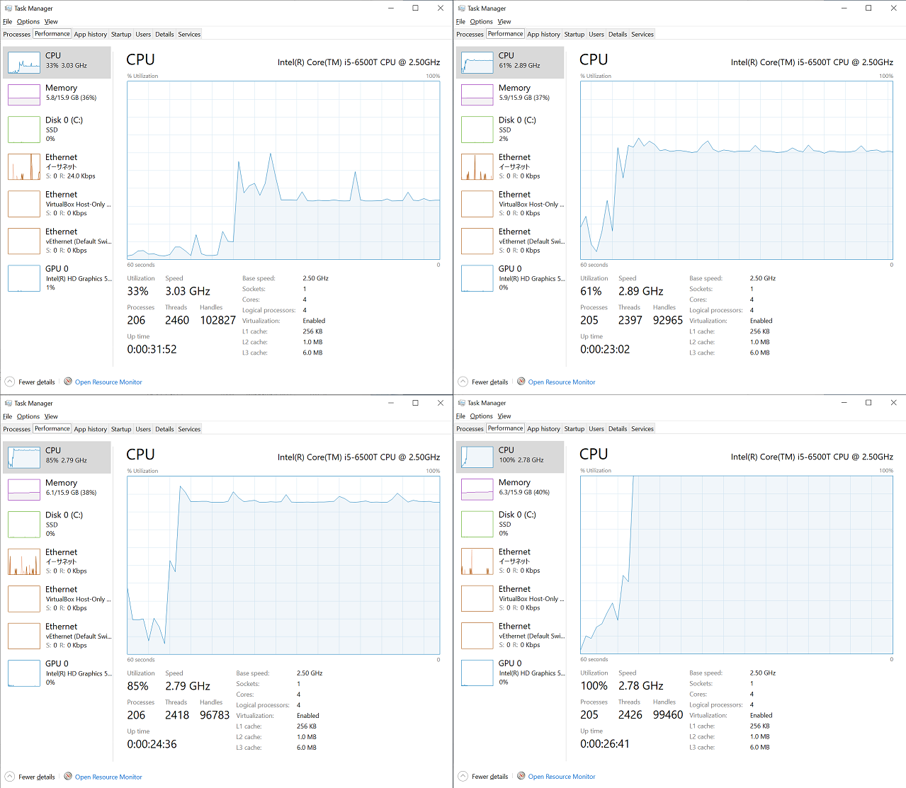
I had captured CPU utilization graphs in Task Manager during each run from the single process run to the 4 process run. As you can see below, about 33% is utilized during the single process run, 60% is utilized during the 2 processes run, 85% during the 3 processes run, and 100% during the 4 processes run, which is in line with my expectation.
Further challenges
Processing 30000 model points in less than 3 minutes on my 5-year-old consumer PC is not impractically slow at all. But keep in mind that fastlife is simpler than most production models. It should also be noted that fastlife is an annual projection model with 100 time steps, so for monthly models, computational load would be 12 times more.
I could further improve the performance of fastlife, but probably I won’t because optimization techniques would be specific to the fastlife model and not applicable to other models.
In the context of multiprocessing, sharing common data in memory across processes is a challenge to tackle. Python has a standard library for shared memory, but only data of primitive types can be shared.
Another challenge is memory consumption. modelx stores all the intermediate values needed to calculate the end results that the user requested, which would lead to massive memory consumption if the model is given a large model points.